Tiskarstvo 03

IARIGAI Dubrovnik – Cavtat 2003, Croatia – Advances in printing science and technology: proceedings of the 30 th International iarigai Research Conference; UDK 655:004.91 > (063); 004.91:655 > (063); ISBN 953-96276-6-4 (tvrdi uvez); ISBN 953-96276-7-2 (meki uvez), Acta Graphica Publishers

The stohastic model of simulation of a virtual printing-house

Zoran Nježić, Vilko Žiljak, Klaudio Pap, Blaž Sviličić

Faculty of Graphic Arts, University of Zagreb
Getaldićeva 2, Zagreb, Croatia
zoran.njezic@sk.hinet.hr

1. Introduction

The paper creates and analyses stochastic models [2] that simulate a virtual printing house and its parts. The entire production process is being simulated in order to create extreme risk situations and thereby define maximum production capacities of the system. The simulation in the paper precisely determines bottle-necks. Optimal and highly balanced parameters of graphic production are being created on the basis of measurements and result analysis. Processes are transparent and complex, and each is accompanied by a level of probability and stochastic, thereby introducing modeling of a graphic system [6] [7] as a successful method for improving and optimizing production. There is a new approach to the observation and evaluation of graphical production processes, from preparation to finalization. In the long run, this is reflected in an increase in production, a more stable production line and better use of existing digital equipment.

2. Enhancement of graphic system by simulation methods

Simulation [1][5] enables the creating of extreme conditions in graphic production processes that would cause great damage in the real system. These borderline conditions are the ones in which simulation provides the insight and experience we use to create new ways of organizing production [10]. It is simulation that has showed us the bad sides of management and pure use of printing processes. In order to revive implementation CIP3, i.e. CIP4 in the graphic system [8] it is imperative to establish a more optimized production line. To establish such an approach in practice, it is necessary to reorganize the existing production plants entirely, especially in the sense of enhancing existing know-how and skills.
Hybrid solutions naturally spring to mind [9] for the creation of a competitive product, but the final realization is not possible as long as there is no definition of a stable production line. Significant steps have been made in that area, but for the idea of a hybrid system to take hold, further investigations and adjustments of production processes will be necessary. Simulation methods can also penetrate and describe in detail the state of the graphic system and thus significantly improve and develop the existing know-how in that area.
Such an approach entirely changes previous methods of production management, which in the end results in a more stable production process, instant detection of bottle-neck that leads to delays and in enhanced productivity. The results of such observation can successfully be integrated in the enhancement of hybrid graphic systems and in aiding the development of CIP3 and CIP4 in the sense of a more transparent expansion of the graphic process.
The design of a new graphic product today incorporates several production technologies, which asks for a new approach in product manufacture. Printing-houses must be very flexible in regard to the market environment when it comes to offering quality solutions. Such a new understanding of the market leads to the introduction of new modeling and simulation methods, as well as having expert and consulting teams look for new solutions.
Expert teams are expected to define the flow of information making maximum use of the Internet technology linked to hybrid printing systems. As there is an unlimited number of solutions and unforeseen situations, the simulation method provides optimal solutions along with presumed problems in the real system. Thus one will not only try to foresee market demands on the one hand, but also create a dynamic system on the other hand that will shortly lead to a new graphic product.
Introduction of simulation into graphic systems enhances the flexibility and adaptability of new solutions in printing, finds production delays, critical spots that lead to deadlock and, most importantly, betters the education of production staff.
At the moment there is a very limited number of simulation applications in the market, which points towards the complexity and price of manufacturing such a virtual system. The solutions on offer enable us to learn and train for special situations just as with real graphic machines, only without the enormous cost in material and time. Furthermore, simulators can create extreme situations that can cause damage in the real environment. It is necessary to create as many various educational tools as possible to simulate the system, the printing process, specially ordered situations and individual production sequences. This will also create a new method of education on all levels.
The unpredictability and dynamism of the market brings printing-houses in a position in which they have to hire consulting and expert teams that will suggest new guidelines in information processing. If the printing-house discovers new situations independently within its own plant, it can easily lead to disorganization and jamming. In such a situation, simulators create solutions and suggest production processes that are definitely cheaper than activating the entire printing line. The area of modeling, simulation and virtual reality introduces a new education method for generations to come.
The next step is the organization of information flow and structure within the graphic system. The definite need to adjust to the Internet environment leads to the adaptation to new standards. XML is suggested as a standard, which linked with XSL provides filtered, targeted information [8]. It is also necessary to conduct further research into the behavior of a graphic system supported by such a model. Only after positive results on the stability of the system are obtained can one proceed with a complete implementation of the Internet environment into printing.

2.1. Defining stochastic models

Simulation of graphic production and the evaluation of its successfulness are practically just starting. Research is directed towards stochastic simulation [2] through data analysis [3] of real systems in printing. Processes are open, and because of the level of probability and chance, models are defined as discrete and stochastic.

2.1.1. Experimental development of model of graphic prepress

This stochastic model tries to present and explore the problem on the level of prepress graphic production. For the analysis and evaluation of success special attention has been paid to the areas of digitalization of originals, editing originals, composition of the graphic page and platesetting. Depending on the output final size of the original and the category of editing and composition, every working place is dependent on various time intervals for editing. It has been defined that one third enters the production cycle every four (4) minutes, the second third every (5) minutes, and the rest every six (6) minutes. The digitalization of the original depends on the output file size, so that it takes three minutes for the first 25% of the originals, 3.5 minutes for the next 25%, and 4 minutes for the remaining 50%. The digitalization parameter for the original varies, so that the observation and research of the system will be guided by that very variable. To edit the originals it takes eight (8) minutes for the first third, nine (9) minutes for the second third and ten (10) minutes for the rest. Page composition takes twelve (12) minutes for 25% of the situations, fifteen (15) minutes for the next 45% and twenty (20) minutes for the rest. The model also takes into consideration errors that are unavoidable in editing, so that a certain amount undergoes re-editing defined by control within the production cycle (Figure 1).

Figure 1

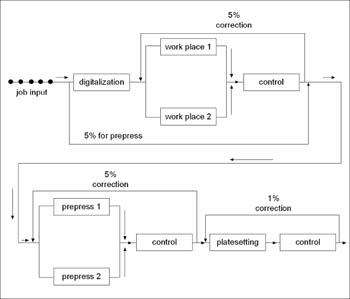
Variable digitalization parameter defined by times:
Time 1: 25% by 1 min, 25% by 1.5 min and 50% by 2 min = experiment A;
Time 2: 25% by 2 min, 25% by 2.5 min and 50% by 3 min = experiment B;
Time 3: 25% by 3 min, 25% by 3.5 min and 50% by 4 min = experiment C;
Time 4: 25% by 4 min, 25% by 4.5 min and 50% by 5 min = experiment D;
Time 5: 25% by 5 min, 25% by 5.5 min and 50% by 6 min = experiment E;
Time 6: 25% by 7 min, 25% by 8.0 min and 50% by 9 min = experiment F.

2.1.2. Experimental development of model of digital printing house

Within the real system there is an unlimited number of multifaceted work-influx variations. This stochastic model describes the printing part in the area of small press runs. Of the entire amount of printing jobs, 25% are runs of 50-150 sheets, 35% are runs of 151-250 sheets, and the remaining 40% are runs of 251-400 sheets. The time necessary for editing and printing preparation is 35 minutes for 30% of the jobs, 55 minutes for 40% of the jobs, and 80 minutes for the remaining 30% of the jobs. The editing parameter varies, so that the cost-effectiveness of the graphic system will be simulated by changing the parameter. The critical borderline area will also be shown, which is hard to reach within the real system, because of a possible crash-down of the entire production unit configuration. Along with the simulation model, there is also an amount taken into consideration that undergoes re-editing after the control process, not only after preparation, but also after printing. Printing speed is set to 150 sheets per minute. The model also takes into account errors during editing and printing, so that a certain amount, i.e. errors unavoidable in the production cycle, undergoes re-editing (Figure 2).

Figure 2

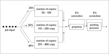
The variable editing and printing parameter defined by times:
Time 1: 30% by 1 min, 40% by 3 min, 30% by 5 min = experiment A;
Time 2: 30% by 7 min, 40% by 10 min, 30% by 15 min = experiment B;
Time 3: 30% by 15 min, 40% by 20 min, 30% by 25 min = experiment C;
Time 4: 30% by 25 min, 40% by 30 min, 30% by 45 min = experiment D;
Time 5: 30% by 40 min, 40% by 45 min, 30% by 50 min = experiment E;
Time 6: 30% by 35 min, 40% by 50 min, 30% by 80 min = experiment F;
Time 7: 30% by 15 min, 40% by 45 min, 30% by 110 min = experiment G.

3. Experimental part

The resource has been used optimally if the utilization is between 70 and 85% [4]. Utilization exceeding 85% very quickly and abruptly leads to a complete deadlock. Digitalization time is taken as variable data in the model (Figure 1) and has been defined by times of 1, 2, 3, 4, 5 and 7 minutes for 25% of the input, by 1.5, 2.5, 3.5, 4.5, 5.5 and 8 minutes for the next 25%, and by 2, 3, 4, 5, 6 and 9 minutes for the remaining 50%. Digitalization times are distributed according to discrete function defined by the described set values. The first case of digitalization time distribution, e.g., is 1 minute for 25% of the jobs, 1.5 minutes for another 25% of the jobs and 2 minutes for the remaining 50%. The extreme case is defined by 7 minutes for 25%, 8 minutes for another 25% and 9 minutes for the remaining 50%. These times present data from the real system, where jobs are defined by several clients. Figure 3 shows simulation results obtained by the above data.

case1= utilization of digitalization;
case2= utilization of control after prepress;
case3= utilization of platesetting;
case4= utilization of editing work place;
case5= utilization of prepress.
Experiments A, B, C, D, E and F present defined times described by discrete function.

Figure 3

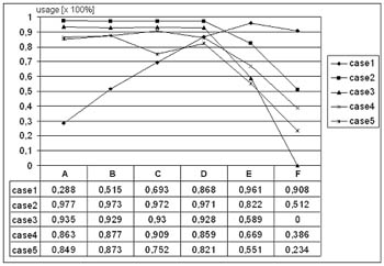
In time intervals the curve for case 1 shows utilization from 28.8% for the shortest digitalization time to 84.9% for the extreme digitalization time case as defined by discrete function. Control after prepress (case 2) was longest at short job in arrival intervals (1, 2, 3, 4, 5 minutes) between 97.7% and 97.1% and became shorter only in time intervals longer than 5 minutes. Control is defined by 9 minutes with 1-minute oscillation. Similarly, in case 3 during short time intervals there was utilization between 86.3 and 90.9%, which became shorter only in time intervals longer than 5 minutes. This point is defined by 15 minutes with 1-minute oscillation. Editing (case 4) was taking place in two work places, because one was totally jammed. There is also a significant drop (38.6%) in time intervals longer than 7 minutes. Layout was divided among two work places (case 5) because of accumulation and queuing.

Optimal use of the digitalization point (case 1) are 69.3% and 86.8% in defined original input times of 3, i.e. 4 minutes for 25% of incoming jobs, 3.5, i.e. 4.5 minutes for another 25% and 4, i.e. 5 minutes for the remaining 50%. This is apparent in experiments C and D. Analyzing the editing working place (case 4), the optimum is achieved at a defined original input time of every 5 minutes for the first 25%, every 5.5 minutes for the next 25% and every 6 minutes for the remaining 50%. It can be said that the platesetting point (case 3) is under great job-influx strain (more than 90%). We suggest the installation of a new platesetter or a new RIP. In experiments C, D and E optimum results were achieved for the described model. In experiment F, when the digitalization is overloaded, one active work place is sufficient.
Figure 4 shows job inputs without a waiting period (percent of zeros). It regards jobs realized directly, without delay and sent to another point. Times used in the simulation are identical to the ones in Figure 3. Figure 4 shows simulation results obtained by that data.
case1= percentage of jobs with no waiting period for editing;
case2= percentage of jobs with no waiting period for digitalization;
case3= percentage of jobs with no waiting period for post-prepress control;
case4= percentage of jobs with no waiting period for prepress.

Figure 4

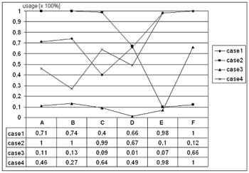
In picture editing there was no waiting period only in time intervals exceeding 5 minutes (98% and 100%). In such situations, if constant, it is possible to have only one work place. This paper does not analyze such a situation in detail. As regards control, one work place is sufficient and 66% of jobs is the highest percentage of jobs realized with no waiting period in intervals of 7, 8 and 9 minutes defined according to described function.

Figure 5

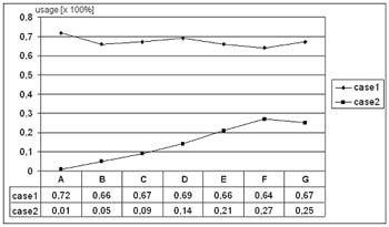
The variable of prepress time, was used as variable data in the model (Figure 2). Prepress times are defined through discrete function as 1, 7, 15, 25, 40, 35, and 15 minutes for 30%, 3, 10, 20, 30, 45, 55 and 45 minutes for 40% and 5, 15, 25, 40, 50, 80 and 110 minutes for the remaining 30%. For the first case of prepress time distribution, editing lasted 1 minute for 30%, 3 minutes for 40% and 5 minutes for the remaining 30%. Printing speed was defined at 150 sheets per minute. Figure 5 shows simulation results.
case1= utilization of digital printing;
case2= utilization of prepress.
Experiments A, B, C, D, E, F and G present defined times described through discrete function.

Optimal utilization of printing (case 1) occurred when job arrival time was defined as 1 minute for 30%, 3 minutes for 40% and 5 minutes for the remaining 30%. Observing total case 1 utilization, we find that it was smallest at 64% in experiment F and largest at 72% in experiment A. The utilization of the prepress work-place (case 2) is so small that the work-place needs to given a higher job arrival frequency.

4. Suggested result presentation for simulation experiment through XML technology

The researcher has to perform hundreds of simulation experiments with the program model. Each experimental simulation measurement result has little value in itself. Only after a larger number of experimental results can certain conclusions be made.
All simulation research into parts of the model has to have several experimental plans. All measurement results have to be placed in a relational database immediately after the experiment (SQL Server, Informix, DB2, Oracle or MSAccess). Each experiment presents one record in the table of experiments. Thus noted data can be obtained in XML format via a previously defined XML Scheme. Here we suggest a design of the XML document for the analysis of targeted resources for six experimental plans A, B, C, D, E and F:

Such an XML document containing all experimental data can easily be filtered and presented using XSL technology. Using XSL Transformation, e.g., one can obtain a new XML document containing only elements with util child element within interval (0.70, 0.85).

5. Conclusion

Research results lead to the conclusion that the simulation method of graphic processes gives both quality and quantity results which are of great use in solving production problems. Problems that occur are linked with insufficient use of individual components, impossibility of testing production in extreme conditions and worker education. The paper elaborates on the production situation of a virtual printing house, based on stochastic models and driven to borderline utilizations. A suggestion has been made for optimal use and new territory has been marked for further development in the graphic engineering domain, especially regarding the concept of virtual production components in printing. By experimenting in simulation, quantity results are obtained defining the use of the resource, pointing towards closing or opening new work places and investing in new hardware or software. The results have shown that there is great discrepancy between components in graphic production workflows. Stochastic models provide highly useful results for solving such problems. A XML method has been suggested for the description of experimental results in order to facilitate future analysis with XSL technology, providing the use of a relational database.

6. Literature references

1. B.P.Zeigler, (1976), Theory of Modelling and Simulation", John Wiley & Sons, USA, ISBN 0-471-98152-4
2. H. Maisel, G. Gnugnoli, (1972), Simulation of Discrete Stochastic Systems", Science Research Associates Inc., USA, ISBN 72-807-61
3. J.P.C. Kleijnen, (1974), Statistical Techniques in Simulation, Marcel Dekker, New Yor, ISBN 0-8247-6157-X
4. K. Pap, V. Žiljak, (2000), Model simulacije dinamičkog konfiguriranja grafičkih sustava, IV simpozij Modeliranje u znanosti, tehnici i društvu., Rijeka 2000. UDK 519.8(082), ISBN 953-6065-00-2
5. V. Žiljak, (1982), Simulacija računalom", Školska knjiga, Zagreb 6. V. Žiljak, K. Pap, (1999), Optimization of individualized reproduction in long-run digital printing, IARIGAI 26th research Conference, Munich 7. V. Žiljak, K. Pap, (1999), Production Management for the Long Run Digital Print with Individualization based on Dinamic Modular Print, 30 th annual Conference of the IC, Stockholm 8. V. Žiljak, K. Pap, D. Agić, I. Žiljak, (2002), Modelling and Simulation of Integration of Web system, Digital and Conventional Printing, 29th International Research Conference of IARIGAI, Lake of Lucerne, Switzerland
9. V. Žiljak, V. Simovic, K. Pap, (2002), Simulation of Stohastic System of Printing Procedures, The International Conference on Modeling and Simulating of Complex System, ICMSCS 2002, Chengdu, China
10. Z. Nježić, V. Žiljak, K. Pap, (2002), Design of Digital Graphic System, International Design Conference DESIGN 2002, pp 876, Dubrovnik, Croatia